Same Training Loss, Different Behavior: Which Solution Should We Choose?

[Cross-posted from smasiha.github.io, Saeed Masiha’s personal blog.]

Which data should an LLM learn from? Answering that question means evaluating the models training produces. But a training objective can leave more than one solution to choose from.

The challenge: equal training loss can hide different outcomes

Minimizing training loss may leave many solutions, with different validation performance. Training alone does not tell us which solution should guide the next update. In this toy example, gradient descent from different initializations approaches different points on the same set of training solutions.

A curved set of training-loss minimizers with three gradient-descent paths ending near different solutions A, B and C, followed by a separate comparison of illustrative validation scores. — Both axes in the landscape are model parameters. The blue curve is the set of training-loss minimizers, and background color shows training loss. Dashed paths are computed gradient-descent runs from different initializations, all with step size 0.16. Their losses approach zero, but their illustrative validation scores differ. In the separate bar chart, each bar corresponds to a model on the curve; height is a validation score, not a count. B scores highest among the sixteen models shown. Explore the original animation.

How this toy example is computed

The loss is

\[g(x)=\frac{1}{2}\bigl(x_2-h(x_1)\bigr)^2,\]

where \(h\) is a smooth cubic interpolation of the curve in my presentation. Its graph is the blue set of zero-loss solutions. The background and paths use this same loss.

Each run uses

\[x_{k+1}=x_k-\eta\nabla g(x_k),\]

with \(\eta=0.16\) for 120 steps. The three initializations are chosen so the runs approach A, B and C. Their final losses are below \(10^{-16}\); the paths are computed without projecting onto the curve.

The validation scores are schematic values from the presentation, not experimental measurements. This illustrates dependence on initialization; it does not assert convergence for every starting point or step size. The scores could represent a shifted negative validation loss, so maximizing them is consistent with minimizing the outer objective.

The curve represents a set of solutions, not an optimization trajectory. The geometry and scores are illustrative, not measured LLM results; the diagram alone does not establish the theorem’s assumptions or identify the best point over the entire continuous curve.

The challenge is to make that choice part of the optimization.

Select, then differentiate

We propose a select-then-differentiate template [1]: first choose a training solution using the objective we ultimately care about, then compute the hypergradient at that selected solution to guide the outer update.

For LLM data reweighting, our practical method explores candidate LoRA updates [2], selects the one with the lowest validation loss, then differentiates through that update to adjust the training-data mixture.

Data-source weights determine training proportions. Four candidate LoRA parameter updates are evaluated on the same validation examples. The candidate with the lowest validation loss guides the next update of the source weights. — Learning which data to emphasize: explore candidate parameter updates, evaluate them on held-out data, select the lowest validation loss, and update the source weights. Network icons represent finite LoRA updates, not exact minimizers. Source proportions and validation-loss bars are illustrative; they are not recorded experimental results. Watch the selection-and-update loop. Implementation details.

Selection happens while learning the data mixture. The resulting mixture is then used for final fine-tuning, before the model is evaluated on test questions.

The template, in formulas

Here \(x\) denotes model parameters; \(\theta\) controls source proportions \(p(\theta)=\operatorname{softmax}(\theta)\).

1. Define training and validation losses

\[g(\theta,x)=\sum_s p_s(\theta)L_s(x), \qquad f(x)=L_{\mathrm{val}}(x).\]

\(L_s\) is the average loss on source \(s\); \(L_{\mathrm{val}}\) is the held-out validation loss.

2. Select using validation loss

\[\mathcal S(\theta)=\operatorname*{arg\,min}_x g(\theta,x),\] \[x^\star(\theta)\in \operatorname*{arg\,min}_{x\in\mathcal S(\theta)} f(x).\]

Among training minimizers, choose the model with the lowest validation loss.

3. Differentiate at the selected solution

\[F(\theta)=f\bigl(x^\star(\theta)\bigr),\] \[\nabla_\theta F =-\nabla_{\theta x}^2 g\, \bigl[\nabla_{xx}^2 g\bigr]^\dagger \nabla_x f.\]

Evaluate every derivative at \((\theta,x^\star(\theta))\). The formula translates the validation gradient through the training curvature into a gradient for the mixture controls. The dagger \((\dagger)\) denotes the pseudoinverse, which handles flat training directions.

Here validation loss has no direct dependence on \(\theta\). The exact formula holds under the paper’s local Polyak–Łojasiewicz and regularity assumptions, including a unique validation-optimal selection for nearby \(\theta\). The LLM implementation uses finite candidate updates as a practical approximation.

What changed in practice?

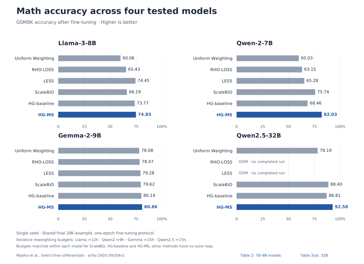
Higher math accuracy across four tested models. HG-MS, our select-then-differentiate method, achieved the highest reported GSM8K and MATH accuracy among completed runs on all four models. Below is the GSM8K comparison; the full results include both benchmarks.

GSM8K test accuracy for six methods on Llama-3-8B, Qwen-2-7B, Gemma-2-9B and Qwen2.5-32B. HG-MS has the highest reported accuracy among completed runs on each model. — GSM8K test accuracy, with a shared 0–100% scale. Single-seed results; OOM means the method ran out of memory under the reported setup, not a zero score. Sources: Table 2 and Table 3(a). View the original comparison.

Full results and experimental protocol

Both benchmarks report test accuracy (%); higher is better. OOM denotes an out-of-memory run. These are single-seed measurements (seed 2424), not averages or evidence of statistical significance.

Llama-3-8B

Method	GSM8K	MATH
Uniform Weighting	60.06	30.24
RHO-LOSS	65.43	25.89
LESS	74.45	29.93
ScaleBiO	66.19	30.58
HG-baseline	73.77	30.49
HG-MS (ours)	74.85	30.86

Qwen-2-7B

Method	GSM8K	MATH
Uniform Weighting	60.03	30.26
RHO-LOSS	63.15	33.40
LESS	65.28	29.24
ScaleBiO	75.74	36.93
HG-baseline	68.46	34.27
HG-MS (ours)	82.03	38.98

Gemma-2-9B

Method	GSM8K	MATH
Uniform Weighting	78.08	37.29
RHO-LOSS	78.47	37.35
LESS	79.28	38.00
ScaleBiO	79.62	37.98
HG-baseline	80.14	38.23
HG-MS (ours)	80.86	38.48

Qwen2.5-32B

Method	GSM8K	MATH
Uniform Weighting	78.19	43.30
RHO-LOSS	OOM	OOM
LESS	OOM	OOM
ScaleBiO	88.40	51.29
HG-baseline	86.81	46.82
HG-MS (ours)	92.58	53.32

The compared methods include RHO-LOSS [3], LESS [4], and ScaleBiO [5]. All numerical results shown here come from our paper [1].

Each completed run uses a final 20,000-example fine-tuning set and one training epoch, with a common evaluation protocol within each model. These are the paper’s adapted baseline implementations under a single-H100 setup.

For the iterative methods (ScaleBiO, HG-baseline, and HG-MS), reweighting time is matched within each model: approximately 12 hours for Llama-3-8B, 9 for Qwen-2-7B, and 15 for Gemma-2-9B and Qwen2.5-32B. The noniterative baselines have no outer reweighting horizon. Experimental protocol.

Download both benchmarks (CSV) · Download the GSM8K figure (SVG)

A closer look: Qwen-2-7B

HG-MS reached 82.03% GSM8K accuracy, compared with 75.74% for ScaleBiO, the strongest comparator here. Its learned mixture also emphasized a different source: DART-Math rather than MathInstruct.

The three iterative methods below use the same ten-source portfolio and nine-hour reweighting budget. Each final mixture supplies 20,000 examples for one epoch of fine-tuning.

Final Qwen-2-7B source mixtures: ScaleBiO and HG-baseline each assign 99.6% to MathInstruct, while HG-MS assigns 94.0% to DART-Math, 5.6% to MathInstruct and 0.4% to Orca-Math. — Same ten sources, different final mixtures. These are final sampling weights, rounded as reported. Each ring totals 100%. The remaining 0.4% is grouped for the comparators; DART-Math's individual comparator weight is not reported. Source: Table 14. View the original diagram.

Source weights and comparison details

All three runs use the same ten-source portfolio and nine-hour reweighting budget. These are sampling weights, not exact counts of sampled examples. For the comparators, the remaining weight is grouped as “remaining sources”. DART-Math’s individual weight is not reported for either comparator; it is included in that remainder, not assumed to be zero.

The top three weights reported in Table 14 are:

Method	Source	Weight (%)
ScaleBiO	MathInstruct	99.6
ScaleBiO	SlimOrca	0.1
ScaleBiO	GPT4-LLM-Cleaned	0.1
HG-baseline	MathInstruct	99.6
HG-baseline	GPT4-LLM-Cleaned	0.3
HG-baseline	SlimOrca	0.0
HG-MS	DART-Math	94.0
HG-MS	MathInstruct	5.6
HG-MS	Orca-Math	0.4

HG-MS’s 0.4% Orca-Math share is shown at the reported precision. A rounded 0.0 does not establish an exactly zero weight. This single-seed comparison does not imply that DART-Math is best for every model, or separate the mixture’s effect from the rest of the procedure.

Download reported source weights (CSV) · Experimental protocol

The mathematical idea

Under the paper’s local regularity assumptions, including its Polyak–Łojasiewicz condition, a unique best choice on the training-solution manifold makes the outer objective locally differentiable even when training has many minimizers. A pseudoinverse gives the corresponding hypergradient. See the precise assumptions and result.

The LLM implementation uses practical finite-step branches; the exact-selection theory does not establish guarantees for those experiments. Theory and practice.

When training leaves a choice, selection becomes part of optimization.

Read Select-then-differentiate: Solving Bilevel Optimization with Manifold Lower-level Solution Sets, joint work with Zebang Shen, Negar Kiyavash, and Niao He, accepted at NeurIPS 2026.

References

[1] Saeed Masiha, Zebang Shen, Negar Kiyavash, and Niao He. Select-then-differentiate: Solving Bilevel Optimization with Manifold Lower-level Solution Sets. NeurIPS, 2026.
[2] Edward J. Hu, Yelong Shen, Phillip Wallis, Zeyuan Allen-Zhu, Yuanzhi Li, Shean Wang, Lu Wang, and Weizhu Chen. LoRA: Low-Rank Adaptation of Large Language Models. ICLR, 2022.
[3] Sören Mindermann, Jan M. Brauner, Muhammed T. Razzak, Mrinank Sharma, Andreas Kirsch, Winnie Xu, Benedikt Höltgen, Aidan N. Gomez, Adrien Morisot, Sebastian Farquhar, and Yarin Gal. Prioritized Training on Points that are Learnable, Worth Learning, and not yet Learnt. ICML, PMLR 162:15630–15649, 2022.
[4] Mengzhou Xia, Sadhika Malladi, Suchin Gururangan, Sanjeev Arora, and Danqi Chen. LESS: Selecting Influential Data for Targeted Instruction Tuning. ICML, PMLR 235:54104–54132, 2024.
[5] Rui Pan, Dylan Zhang, Hanning Zhang, Xingyuan Pan, Minrui Xu, Jipeng Zhang, Renjie Pi, Xiaoyu Wang, and Tong Zhang. ScaleBiO: Scalable Bilevel Optimization for LLM Data Reweighting. ACL, pp. 31959–31982, 2025.